Will the patient show up?
Build, in one notebook, a model that predicts which patients will miss a medical appointment, and turn it into a call list using real costs. Then see the same code become a tested, monitored API.
pandas scikit-learn matplotlib kagglehub, then open the notebook in Jupyter or VS Code.Set up
One place for every import and setting. Fixing the random seed makes every run reproducible.
import warnings
from pathlib import Path

import matplotlib.pyplot as plt
import numpy as np
import pandas as pd
import sklearn

assert tuple(map(int, sklearn.__version__.split(".")[:2])) >= (1, 6), (
    "needs scikit-learn 1.6+: pip install -U scikit-learn"
)
warnings.filterwarnings("ignore", category=FutureWarning)
pd.set_option("display.max_columns", 30)
plt.rcParams.update({"figure.dpi": 110, "axes.spines.top": False, "axes.spines.right": False})

SEED = 42
print("scikit-learn", sklearn.__version__)
scikit-learn 1.9.1
Frame the problem
Before touching data, write down who uses the model, what decision it supports, and what a mistake costs.
| User | Clinic reception staff, each afternoon |
| Decision | Which of tomorrow's (and later) patients to phone with a reminder |
| Prediction time | When the appointment is booked, using only what is known then |
| Not for | Refusing, delaying or overbooking care for anyone |
A call costs staff time; a missed appointment wastes a slot. With rough costs agreed with the clinic, we can work out when a call is worth making: a call pays off when probability of no-show × share of no-shows a call prevents × value of the slot is larger than the cost of the call.
COST_OF_CALL = 5.0  # AUD of staff time per reminder call
COST_OF_NO_SHOW = 60.0  # AUD value of a wasted slot
CALL_PREVENTS = 0.30  # share of would-be no-shows that a call turns into attendance

break_even = COST_OF_CALL / (CALL_PREVENTS * COST_OF_NO_SHOW)
print(f"A call is worth it when the no-show probability is above {break_even:.3f} ({break_even:.1%})")
A call is worth it when the no-show probability is above 0.278 (27.8%)
That number is the decision threshold, set by the business before we see any model. It also tells us that probabilities must be accurate (calibrated), not just good at ranking, because we compare them to 27.8%.
Load the data
The real data is the Kaggle Medical Appointment No Shows dataset (110,527 appointments in Vitória, Brazil, 2016,
licence CC BY-NC-SA 4.0). The next cell looks for the CSV next to the notebook, otherwise downloads it with
kagglehub (preinstalled in Colab; if it asks you to sign in, add a free Kaggle API key, or download the CSV from the
Kaggle page and drag it into Colab's Files panel).
If neither works, for example with no internet, it falls back to practice data: a synthetic table with the same columns, the same quirks and similar patterns, made by the function below. Never report numbers from practice data.
def make_practice_data(rows=110_527, seed=SEED):
    """Synthetic appointments with the real file's columns and quirks (for practice only)."""
    rng = np.random.default_rng(seed)
    hoods = [f"BAIRRO {i:02d}" for i in range(1, 41)]
    n_patients = max(50, int(rows * 0.56))
    pat_ids = rng.integers(10**11, 10**15, n_patients).astype(float)
    pat_age = np.clip(rng.gamma(2.2, 17.0, n_patients).round(), 0, 110).astype(int)
    pat_gender = rng.choice(["F", "M"], n_patients, p=[0.65, 0.35])
    pat_hood = rng.choice(len(hoods), n_patients, p=np.random.default_rng(1).dirichlet(np.ones(len(hoods))))
    pat_tendency = rng.normal(0, 0.9, n_patients)  # unobserved: some patients miss more often
    pat_scholar = rng.random(n_patients) < 0.10
    pat_hyper = rng.random(n_patients) < np.clip(pat_age / 140, 0, 0.6)
    pat_diab = rng.random(n_patients) < np.clip(pat_age / 400, 0, 0.2)
    pat_alc = rng.random(n_patients) < 0.03
    pat_hand = rng.choice([0, 1, 2, 3, 4], n_patients, p=[0.979, 0.018, 0.0025, 0.0004, 0.0001])

    who = rng.choice(n_patients, rows, p=None)
    appt = pd.Timestamp("2016-04-29") + pd.to_timedelta(rng.integers(0, 41, rows), unit="D")
    appt = appt.where(appt.dayofweek != 6, appt + pd.Timedelta(days=1))  # no Sunday appointments
    lead = np.where(rng.random(rows) < 0.35, 0, np.ceil(rng.exponential(14, rows))).astype(int)
    sched = (
        appt
        - pd.to_timedelta(lead, unit="D")
        + pd.to_timedelta(rng.integers(7 * 3600, 19 * 3600, rows), unit="s")
    )
    sms = ((lead >= 3) & (rng.random(rows) < 0.55)).astype(int)
    age = pat_age[who]
    z = (
        -1.85
        + 0.022 * np.minimum(lead, 60)
        - 0.012 * (age - 40)
        + 0.35 * pat_scholar[who]
        + 0.3 * pat_alc[who]
        - 0.25 * sms
        + pat_tendency[who]
        + 0.15 * (appt.dayofweek.to_numpy() == 0)
    )
    no_show = rng.random(rows) < 1 / (1 + np.exp(-z))
    df = pd.DataFrame(
        {
            "PatientId": pat_ids[who],
            "AppointmentID": rng.permutation(np.arange(5_000_000, 5_000_000 + rows)),
            "Gender": pat_gender[who],
            "ScheduledDay": sched.strftime("%Y-%m-%dT%H:%M:%SZ"),
            "AppointmentDay": appt.strftime("%Y-%m-%dT00:00:00Z"),
            "Age": age,
            "Neighbourhood": np.array(hoods)[pat_hood[who]],
            "Scholarship": pat_scholar[who].astype(int),
            "Hipertension": pat_hyper[who].astype(int),
            "Diabetes": pat_diab[who].astype(int),
            "Alcoholism": pat_alc[who].astype(int),
            "Handcap": pat_hand[who],
            "SMS_received": sms,
            "No-show": np.where(no_show, "Yes", "No"),
        }
    )
    df.loc[0, "Age"] = -1  # the real file's quirks, so the cleaning rules have something to do
    late = df.index[1:3]
    df.loc[late, "ScheduledDay"] = (
        pd.to_datetime(df.loc[late, "AppointmentDay"]) + pd.Timedelta(days=1, hours=9)
    ).dt.strftime("%Y-%m-%dT%H:%M:%SZ")
    return df
CSV = "noshowappointments-kagglev2-may-2016.csv"
found = next((p for p in (Path(CSV), Path("data") / CSV, Path("../data/raw") / CSV) if p.exists()), None)
if found is None:
    try:
        import kagglehub

        found = next(Path(kagglehub.dataset_download("joniarroba/noshowappointments")).glob("*.csv"))
    except Exception as e:  # no internet, no Kaggle access, or kagglehub not installed
        print(f"could not download the real data ({type(e).__name__})")
if found is not None:
    raw = pd.read_csv(found)
    print(f"loaded {len(raw):,} rows from {found}")
else:
    raw = make_practice_data()
    print(f"using {len(raw):,} rows of synthetic PRACTICE data: do not report these numbers")
raw.head()
could not download the real data (ModuleNotFoundError)
using 110,527 rows of synthetic PRACTICE data: do not report these numbers
| PatientId | AppointmentID | Gender | ScheduledDay | AppointmentDay | Age | Neighbourhood | Scholarship | Hipertension | Diabetes | Alcoholism | Handcap | SMS_received | No-show | |
|---|---|---|---|---|---|---|---|---|---|---|---|---|---|---|
| 0 | 7.342097e+14 | 5099038 | F | 2016-06-04T10:21:39Z | 2016-06-04T00:00:00Z | -1 | BAIRRO 31 | 0 | 0 | 0 | 0 | 0 | 0 | Yes |
| 1 | 2.302251e+14 | 5036345 | F | 2016-05-24T09:00:00Z | 2016-05-23T00:00:00Z | 27 | BAIRRO 23 | 1 | 1 | 0 | 0 | 0 | 0 | Yes |
| 2 | 5.406092e+14 | 5004843 | F | 2016-05-07T09:00:00Z | 2016-05-06T00:00:00Z | 88 | BAIRRO 31 | 0 | 1 | 0 | 0 | 0 | 1 | No |
| 3 | 6.937668e+13 | 5003094 | M | 2016-05-16T07:11:18Z | 2016-05-16T00:00:00Z | 21 | BAIRRO 13 | 0 | 1 | 0 | 0 | 0 | 0 | No |
| 4 | 2.957149e+14 | 5107907 | M | 2016-04-22T16:10:08Z | 2016-05-17T00:00:00Z | 33 | BAIRRO 40 | 0 | 0 | 0 | 0 | 0 | 1 | No |
First look
Check the size, the types and the target before anything else. Note the misspelt column names (Hipertension,
Handcap) in the original data: we will rename them.
print(raw.shape)
raw.dtypes
(110527, 14)
PatientId         float64
AppointmentID       int64
Gender                str
ScheduledDay          str
AppointmentDay        str
Age                 int64
Neighbourhood         str
Scholarship         int64
Hipertension        int64
Diabetes            int64
Alcoholism          int64
Handcap             int64
SMS_received        int64
No-show               str
dtype: object
raw.describe().T.round(2)
| count | mean | std | min | 25% | 50% | 75% | max | |
|---|---|---|---|---|---|---|---|---|
| PatientId | 110527.0 | 4.991562e+14 | 2.881439e+14 | 1.131672e+11 | 2.496144e+14 | 5.001005e+14 | 7.483908e+14 | 9.999937e+14 |
| AppointmentID | 110527.0 | 5.055263e+06 | 3.190654e+04 | 5.000000e+06 | 5.027632e+06 | 5.055263e+06 | 5.082894e+06 | 5.110526e+06 |
| Age | 110527.0 | 3.718000e+01 | 2.411000e+01 | -1.000000e+00 | 1.900000e+01 | 3.200000e+01 | 5.000000e+01 | 1.100000e+02 |
| Scholarship | 110527.0 | 1.000000e-01 | 3.000000e-01 | 0.000000e+00 | 0.000000e+00 | 0.000000e+00 | 0.000000e+00 | 1.000000e+00 |
| Hipertension | 110527.0 | 2.700000e-01 | 4.400000e-01 | 0.000000e+00 | 0.000000e+00 | 0.000000e+00 | 1.000000e+00 | 1.000000e+00 |
| Diabetes | 110527.0 | 9.000000e-02 | 2.800000e-01 | 0.000000e+00 | 0.000000e+00 | 0.000000e+00 | 0.000000e+00 | 1.000000e+00 |
| Alcoholism | 110527.0 | 3.000000e-02 | 1.700000e-01 | 0.000000e+00 | 0.000000e+00 | 0.000000e+00 | 0.000000e+00 | 1.000000e+00 |
| Handcap | 110527.0 | 2.000000e-02 | 1.800000e-01 | 0.000000e+00 | 0.000000e+00 | 0.000000e+00 | 0.000000e+00 | 4.000000e+00 |
| SMS_received | 110527.0 | 3.100000e-01 | 4.600000e-01 | 0.000000e+00 | 0.000000e+00 | 0.000000e+00 | 1.000000e+00 | 1.000000e+00 |
raw["No-show"].value_counts(normalize=True).rename("share")
No-show
No     0.794394
Yes    0.205606
Name: share, dtype: float64
About one appointment in five is missed. That imbalance matters: accuracy would be 80% for a model that always says "will attend", so we will judge models with PR-AUC (average precision) and probability quality instead.
Check data quality
Turn every assumption into a check. Hard problems (missing columns, unknown codes) would stop us; known quirks are counted so we can decide how to handle each one.
sched = pd.to_datetime(raw["ScheduledDay"], utc=True)
appt = pd.to_datetime(raw["AppointmentDay"], utc=True)
checks = pd.Series(
    {
        "missing values": int(raw.isna().sum().sum()),
        "duplicate AppointmentID": int(raw["AppointmentID"].duplicated().sum()),
        "Gender not F/M": int((~raw["Gender"].isin(["F", "M"])).sum()),
        "negative Age": int((raw["Age"] < 0).sum()),
        "Age above 115": int((raw["Age"] > 115).sum()),
        "appointment before booking day": int((appt.dt.normalize() < sched.dt.normalize()).sum()),
        "Handcap above 1 (it is a 0-4 level)": int((raw["Handcap"] > 1).sum()),
        "AppointmentDay with a time other than 00:00": int((appt.dt.hour != 0).sum()),
    },
    name="rows",
)
checks
missing values                                   0
duplicate AppointmentID                          0
Gender not F/M                                   0
negative Age                                     1
Age above 115                                    0
appointment before booking day                   2
Handcap above 1 (it is a 0-4 level)            319
AppointmentDay with a time other than 00:00      0
Name: rows, dtype: int64
Findings: a few impossible ages, some appointments dated before they were booked (data-entry errors), Handcap is
a level from 0 to 4 rather than yes/no, and AppointmentDay has no time of day. Nothing stops us.
Clean the data
Rename and type the columns, then remove rows with named rules, counting what each rule removes so the effect of cleaning is visible.
RENAME = {
    "PatientId": "patient_id",
    "AppointmentID": "appointment_id",
    "Gender": "gender",
    "ScheduledDay": "scheduled_at",
    "AppointmentDay": "appointment_date",
    "Age": "age",
    "Neighbourhood": "neighbourhood",
    "Scholarship": "scholarship",
    "Hipertension": "hypertension",
    "Diabetes": "diabetes",
    "Alcoholism": "alcoholism",
    "Handcap": "handicap_level",
    "SMS_received": "sms_received",
    "No-show": "no_show_raw",
}

df = raw.rename(columns=RENAME)[list(RENAME.values())].copy()
df["patient_id"] = df["patient_id"].astype("int64").astype("string")  # stored as float in the CSV
df["appointment_id"] = df["appointment_id"].astype("int64")
df["scheduled_at"] = pd.to_datetime(df["scheduled_at"], utc=True).dt.tz_localize(None)
df["appointment_date"] = pd.to_datetime(df["appointment_date"], utc=True).dt.tz_localize(None).dt.normalize()
df["gender"] = df["gender"].astype("category")
df["neighbourhood"] = df["neighbourhood"].astype("string").str.strip().str.upper()
for col in ("scholarship", "hypertension", "diabetes", "alcoholism", "sms_received"):
    df[col] = df[col].astype("int8")
df["handicap_level"] = df["handicap_level"].astype("int8")
df["no_show"] = (df.pop("no_show_raw") == "Yes").astype("int8")  # target: 1 = did NOT attend

rules = {
    "negative_age": df["age"] < 0,
    "age_above_max": df["age"] > 115,
    "appointment_before_booking": df["appointment_date"] < df["scheduled_at"].dt.normalize(),
    "duplicate_appointment_id": df["appointment_id"].duplicated(keep="first"),
}
keep = pd.Series(True, index=df.index)
removed = {}
for name, mask in rules.items():
    removed[name] = int((mask & keep).sum())  # each row counted once, under the first rule that removes it
    keep &= ~mask
clean = (
    df.loc[keep].sort_values(["appointment_date", "scheduled_at", "appointment_id"]).reset_index(drop=True)
)
print(f"{len(df):,} rows -> {len(clean):,} rows")
pd.Series(removed, name="rows removed")
110,527 rows -> 110,524 rows
negative_age                  1
age_above_max                 0
appointment_before_booking    2
duplicate_appointment_id      0
Name: rows removed, dtype: int64
Split by time, before exploring
The model will always be trained on the past and used on the future, so we split the same way: the earliest 70% of appointment dates for training, the next 15% for validation (choosing and calibrating the model) and the last 15% for a final test, used once. We split before exploring so that what we see in the test period cannot influence our choices.
counts = clean.groupby("appointment_date").size().sort_index()
share = counts.cumsum() / counts.sum()
validation_start = share.index[(share > 0.70).to_numpy().argmax()]
test_start = share.index[(share > 0.85).to_numpy().argmax()]
period = np.where(
    clean["appointment_date"] < validation_start,
    "train",
    np.where(clean["appointment_date"] < test_start, "validation", "test"),
)
clean.groupby(period, sort=False).agg(
    rows=("no_show", "size"),
    no_show_rate=("no_show", "mean"),
    first=("appointment_date", "min"),
    last=("appointment_date", "max"),
)
| rows | no_show_rate | first | last | |
|---|---|---|---|---|
| train | 75179 | 0.204472 | 2016-04-29 | 2016-05-26 |
| validation | 16229 | 0.206174 | 2016-05-27 | 2016-06-01 |
| test | 19116 | 0.209510 | 2016-06-02 | 2016-06-08 |
Explore the training period
Questions first, then charts. Does waiting longer for an appointment raise the risk? Who misses more? Do SMS reminders help? Everything here uses the training period only.
train_raw = clean[period == "train"].copy()
train_raw["lead_days"] = (train_raw["appointment_date"] - train_raw["scheduled_at"].dt.normalize()).dt.days
overall = train_raw["no_show"].mean()


def rate_by(col, title, ax):
    t = train_raw.groupby(col, observed=True)["no_show"].agg(["mean", "size"])
    ax.bar(t.index.astype(str), t["mean"], color="#2E6FF2")
    ax.axhline(overall, color="#E07B00", ls="--", lw=1)
    ax.set(title=title, ylabel="no-show rate")
    ax.tick_params(axis="x", rotation=45, labelsize=8)
    return t


fig, axes = plt.subplots(2, 2, figsize=(11, 7))
lead_bins = pd.cut(
    train_raw["lead_days"],
    [-1, 0, 2, 7, 14, 30, 60, 400],
    labels=["same day", "1-2", "3-7", "8-14", "15-30", "31-60", "60+"],
)
rate_by(lead_bins, "By days between booking and appointment", axes[0, 0])
age_band = pd.cut(
    train_raw["age"],
    [-1, 12, 17, 34, 49, 64, 200],
    labels=["0-12", "13-17", "18-34", "35-49", "50-64", "65+"],
)
rate_by(age_band, "By age band", axes[0, 1])
rate_by("sms_received", "By SMS reminder received", axes[1, 0])
weekday = pd.Categorical(
    train_raw["appointment_date"].dt.day_name().str[:3], categories=["Mon", "Tue", "Wed", "Thu", "Fri", "Sat"]
)
rate_by(weekday, "By weekday", axes[1, 1])
fig.tight_layout()
plt.show()
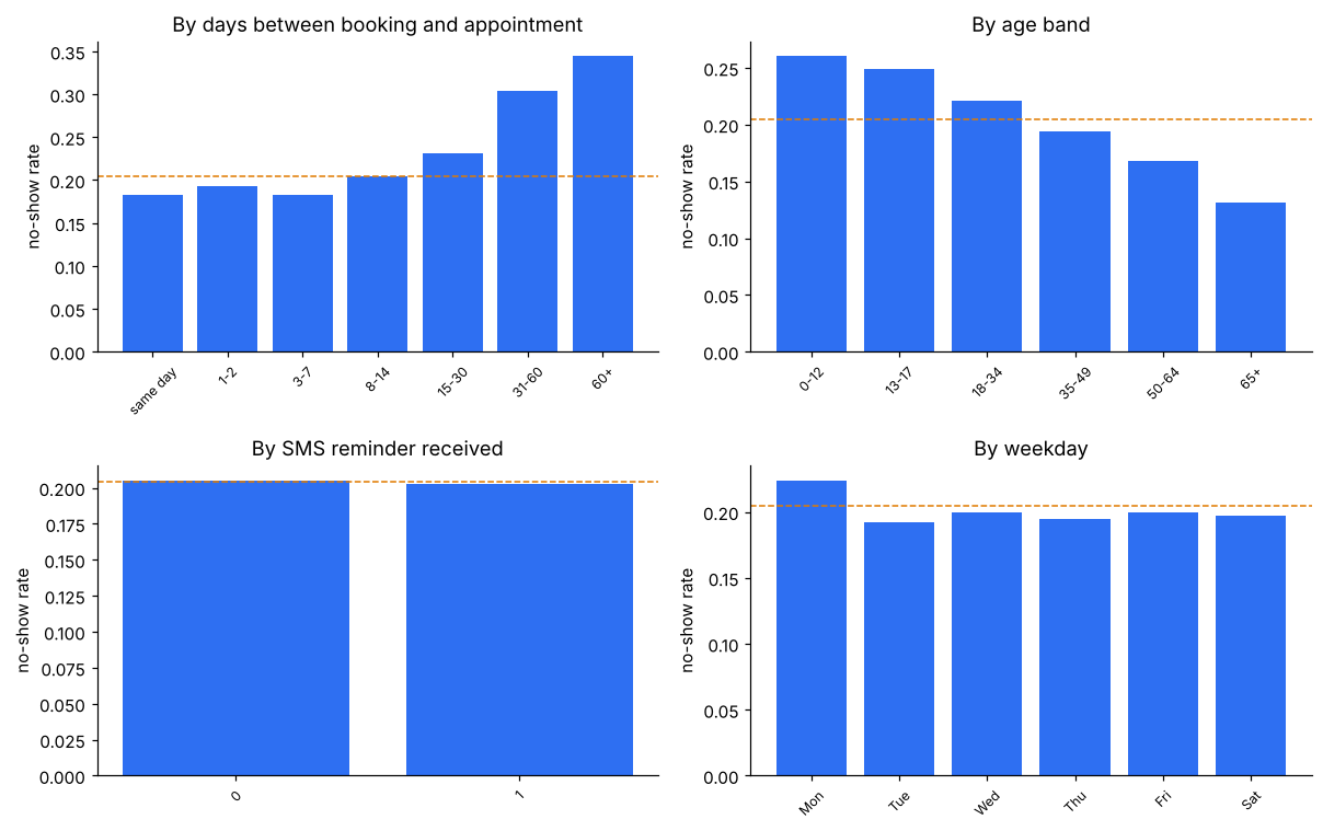
What to look for. The saved charts come from synthetic data; the real data shows these patterns, some more strongly:
-
Lead time is the strongest pattern: risk climbs the longer patients wait. In the real data, same-day appointments are almost always kept.
-
Age: children, teenagers and young adults miss more often than older patients.
- The SMS paradox (real data): patients who received an SMS miss more (about 28% against 17%). SMS were only sent for appointments booked days ahead, so SMS is tangled up with lead time. This is confounding, not proof that SMS backfires, and a reason never to read a model's weights as causes. (The synthetic generator does not reproduce it, so the bar chart above is flat.)
Does past behaviour predict future behaviour? We need each patient's history, but only the part known at booking.
visits = train_raw.groupby("patient_id").size()
print(f"{(visits > 1).mean():.0%} of patients have more than one appointment in the training period")
train_raw.groupby(train_raw.groupby("patient_id").cumcount().clip(upper=3))["no_show"].mean().rename(
    "no-show rate by visit number (3 = 3rd+)"
)
49% of patients have more than one appointment in the training period
0    0.203976
1    0.205288
2    0.205501
3    0.203218
Name: no-show rate by visit number (3 = 3rd+), dtype: float64
Engineer features without leaking the future
Two kinds of features:
- Row features use only the appointment itself (lead time, age, weekday, conditions...).
- History features count the patient's earlier appointments and no-shows, using only appointments whose outcome was known when this one was booked (at least one day before the booking date).
Counting all of a patient's no-shows, including later ones, is a classic leak: it scores brilliantly offline and fails in production.
WEEKDAYS = ["Mon", "Tue", "Wed", "Thu", "Fri", "Sat", "Sun"]


def row_features(d):
    out = pd.DataFrame(index=d.index)
    booked_day = d["scheduled_at"].dt.normalize()
    out["lead_days"] = (d["appointment_date"] - booked_day).dt.days.astype("int32")
    out["same_day"] = (out["lead_days"] == 0).astype("int8")
    out["scheduled_hour"] = d["scheduled_at"].dt.hour.astype("int8")
    out["appointment_weekday"] = pd.Categorical(
        d["appointment_date"].dt.dayofweek.map(dict(enumerate(WEEKDAYS))), categories=WEEKDAYS
    )
    out["age"] = d["age"].astype("int16")
    out["age_band"] = pd.cut(
        d["age"],
        bins=[-1, 12, 17, 34, 49, 64, 200],
        labels=["0-12", "13-17", "18-34", "35-49", "50-64", "65+"],
    )
    out["gender_f"] = (d["gender"].astype("string") == "F").astype("int8")
    out["handicap_level"] = d["handicap_level"].astype("int8")
    for col in ("scholarship", "hypertension", "diabetes", "alcoholism", "sms_received"):
        out[col] = d[col].astype("int8")
    out["n_conditions"] = (
        d["hypertension"] + d["diabetes"] + d["alcoholism"] + (d["handicap_level"] > 0)
    ).astype("int8")
    out["neighbourhood"] = d["neighbourhood"].astype("string")
    return out


def history_features(d, min_days_gap=1):
    """Earlier appointments and no-shows per patient, known at booking time (merge_asof: strictly before)."""
    events = (
        d.groupby(["patient_id", "appointment_date"], observed=True)["no_show"]
        .agg(n="size", ns="sum")
        .reset_index()
        .sort_values("appointment_date")
    )
    events["cum_n"] = events.groupby("patient_id")["n"].cumsum()
    events["cum_ns"] = events.groupby("patient_id")["ns"].cumsum()
    q = pd.DataFrame(
        {
            "row": d.index,
            "patient_id": d["patient_id"],
            "cutoff": d["scheduled_at"].dt.normalize() - pd.Timedelta(days=min_days_gap - 1),
        }
    )
    m = pd.merge_asof(
        q.sort_values("cutoff"),
        events[["patient_id", "appointment_date", "cum_n", "cum_ns"]],
        left_on="cutoff",
        right_on="appointment_date",
        by="patient_id",
        allow_exact_matches=False,
        direction="backward",
    )
    m = m.set_index("row").reindex(d.index)
    out = pd.DataFrame(index=d.index)
    out["prior_appointments"] = m["cum_n"].fillna(0).astype("int32")
    out["prior_no_shows"] = m["cum_ns"].fillna(0).astype("int32")
    with np.errstate(divide="ignore", invalid="ignore"):
        out["prior_no_show_rate"] = (
            out["prior_no_shows"] / out["prior_appointments"].replace(0, np.nan)
        ).astype("float64")
    out["days_since_last_appointment"] = (m["cutoff"] - m["appointment_date"]).dt.days.astype("float64")
    return out


NUMERIC = [
    "lead_days",
    "age",
    "scheduled_hour",
    "n_conditions",
    "handicap_level",
    "prior_appointments",
    "prior_no_shows",
    "prior_no_show_rate",
    "days_since_last_appointment",
]
BINARY = ["same_day", "gender_f", "scholarship", "hypertension", "diabetes", "alcoholism", "sms_received"]
CATEGORICAL = ["appointment_weekday", "neighbourhood"]
FEATURES = NUMERIC + BINARY + CATEGORICAL
META = ["appointment_id", "patient_id", "appointment_date", "scheduled_at", "gender", "age_band"]

feats = pd.concat(
    [
        clean[["appointment_id", "patient_id", "appointment_date", "scheduled_at", "gender"]],
        row_features(clean),
        history_features(clean),
        clean[["no_show"]],
    ],
    axis=1,
)[META + FEATURES + ["no_show"]]
feats[FEATURES].head()
| lead_days | age | scheduled_hour | n_conditions | handicap_level | prior_appointments | prior_no_shows | prior_no_show_rate | days_since_last_appointment | same_day | gender_f | scholarship | hypertension | diabetes | alcoholism | sms_received | appointment_weekday | neighbourhood | |
|---|---|---|---|---|---|---|---|---|---|---|---|---|---|---|---|---|---|---|
| 0 | 135 | 54 | 15 | 0 | 0 | 0 | 0 | NaN | NaN | 0 | 1 | 0 | 0 | 0 | 0 | 1 | Fri | BAIRRO 29 |
| 1 | 134 | 110 | 14 | 1 | 0 | 0 | 0 | NaN | NaN | 0 | 1 | 0 | 1 | 0 | 0 | 0 | Fri | BAIRRO 24 |
| 2 | 88 | 39 | 7 | 1 | 0 | 0 | 0 | NaN | NaN | 0 | 1 | 0 | 0 | 1 | 0 | 0 | Fri | BAIRRO 19 |
| 3 | 80 | 45 | 18 | 2 | 1 | 0 | 0 | NaN | NaN | 0 | 0 | 0 | 1 | 0 | 0 | 0 | Fri | BAIRRO 03 |
| 4 | 74 | 8 | 16 | 0 | 0 | 0 | 0 | NaN | NaN | 0 | 1 | 0 | 0 | 0 | 0 | 1 | Fri | BAIRRO 36 |
Prove there is no leakage. Pick a patient with several visits and check by hand that each history count only includes appointments that ended at least a day before the booking.
pid = feats.loc[feats["prior_appointments"] >= 2, "patient_id"].iloc[0]
one = feats[feats["patient_id"] == pid].sort_values("scheduled_at")
for _, r in one.iterrows():
    earlier = one[one["appointment_date"] < r["scheduled_at"].normalize()]
    assert r["prior_appointments"] == len(earlier) and r["prior_no_shows"] == earlier["no_show"].sum()
one[["scheduled_at", "appointment_date", "no_show", "prior_appointments", "prior_no_shows"]]
| scheduled_at | appointment_date | no_show | prior_appointments | prior_no_shows | |
|---|---|---|---|---|---|
| 3753 | 2016-04-21 12:38:07 | 2016-04-30 | 0 | 0 | 0 |
| 4733 | 2016-04-30 09:14:30 | 2016-04-30 | 0 | 0 | 0 |
| 8761 | 2016-05-01 09:47:53 | 2016-05-02 | 0 | 2 | 0 |
| 44519 | 2016-05-04 10:00:36 | 2016-05-16 | 0 | 3 | 0 |
| 63344 | 2016-05-12 16:00:36 | 2016-05-23 | 0 | 3 | 0 |
Now split the feature table with the same dates as before.
d = feats["appointment_date"]
train, val, test = (
    feats[d < validation_start],
    feats[(d >= validation_start) & (d < test_start)],
    feats[d >= test_start],
)
X_train, y_train = train[FEATURES], train["no_show"]
X_val, y_val = val[FEATURES], val["no_show"]
print(f"train {len(train):,} | validation {len(val):,} | test {len(test):,} (test untouched until the end)")
train 75,179 | validation 16,229 | test 19,116 (test untouched until the end)
Start with a baseline
The simplest possible model predicts the training no-show rate for everyone. Its PR-AUC equals the share of no-shows. Any real model must clearly beat it, or it is not worth the complexity.
Cross-validation folds are grouped by patient: the same patient never appears in both the training and the scoring part of a fold, so a model cannot score well by memorising individuals.
from sklearn.dummy import DummyClassifier
from sklearn.metrics import average_precision_score, brier_score_loss, roc_auc_score
from sklearn.model_selection import GroupKFold

folds = list(GroupKFold(n_splits=5).split(X_train, y_train, groups=train["patient_id"]))


def scores(y, p):
    return {
        "ROC-AUC": roc_auc_score(y, p),
        "PR-AUC": average_precision_score(y, p),
        "Brier": brier_score_loss(y, p),
    }


dummy = DummyClassifier(strategy="prior").fit(X_train, y_train)
results = {"baseline": scores(y_val, dummy.predict_proba(X_val)[:, 1])}
pd.DataFrame(results).T.round(4)
| ROC-AUC | PR-AUC | Brier | |
|---|---|---|---|
| baseline | 0.5 | 0.2062 | 0.1637 |
Model 1: logistic regression
A linear model is fast, explainable and often hard to beat. Preprocessing goes inside the pipeline so it is learned from training folds only and saved with the model:
- numbers: fill missing history with the median, add a "was missing" flag, standardise;
- weekday: one-hot; neighbourhood: one-hot with rare ones grouped as "infrequent".
from scipy.stats import loguniform, randint, uniform
from sklearn.compose import ColumnTransformer
from sklearn.impute import SimpleImputer
from sklearn.linear_model import LogisticRegression
from sklearn.model_selection import RandomizedSearchCV
from sklearn.pipeline import Pipeline, make_pipeline
from sklearn.preprocessing import OneHotEncoder, StandardScaler

logistic = Pipeline(
    [
        (
            "pre",
            ColumnTransformer(
                [
                    (
                        "num",
                        make_pipeline(SimpleImputer(strategy="median", add_indicator=True), StandardScaler()),
                        NUMERIC,
                    ),
                    ("bin", "passthrough", BINARY),
                    (
                        "wday",
                        OneHotEncoder(categories=[WEEKDAYS], drop="first", handle_unknown="ignore"),
                        ["appointment_weekday"],
                    ),
                    (
                        "hood",
                        OneHotEncoder(min_frequency=50, handle_unknown="infrequent_if_exist"),
                        ["neighbourhood"],
                    ),
                ],
                verbose_feature_names_out=True,
            ),
        ),
        ("clf", LogisticRegression(max_iter=3000, random_state=SEED)),
    ]
)
search_lr = RandomizedSearchCV(
    logistic,
    {"clf__C": loguniform(1e-3, 1e2), "clf__class_weight": [None, "balanced"]},
    n_iter=20,
    scoring="average_precision",
    cv=folds,
    random_state=SEED,
    n_jobs=-1,
)
search_lr.fit(X_train, y_train)
print(
    "best:",
    {k: (round(float(v), 4) if isinstance(v, float) else v) for k, v in search_lr.best_params_.items()},
    f"CV PR-AUC {search_lr.best_score_:.4f}",
)
results["logistic"] = scores(y_val, search_lr.predict_proba(X_val)[:, 1])
best: {'clf__C': 0.005, 'clf__class_weight': 'balanced'} CV PR-AUC 0.2821
Model 2: gradient boosting
Trees capture interactions (lead time matters more for young adults) and handle missing history natively. Two details worth copying:
- Target encoding for neighbourhood, cross-fitted so a row's code never uses its own label.
- A monotonic constraint: more past no-shows must never lower the predicted risk. Domain knowledge as a rule makes the model more trustworthy and harder to fool with noise.
from sklearn.ensemble import HistGradientBoostingClassifier
from sklearn.model_selection import KFold
from sklearn.preprocessing import OrdinalEncoder, TargetEncoder

hgb = Pipeline(
    [
        (
            "pre",
            ColumnTransformer(
                [
                    ("num", "passthrough", NUMERIC),
                    ("bin", "passthrough", BINARY),
                    (
                        "wday",
                        OrdinalEncoder(
                            categories=[WEEKDAYS], handle_unknown="use_encoded_value", unknown_value=-1
                        ),
                        ["appointment_weekday"],
                    ),
                    (
                        "hood",
                        TargetEncoder(target_type="binary", cv=KFold(5, shuffle=True, random_state=SEED)),
                        ["neighbourhood"],
                    ),
                ],
                verbose_feature_names_out=True,
            ).set_output(transform="pandas"),
        ),
        (
            "clf",
            HistGradientBoostingClassifier(
                random_state=SEED,
                early_stopping=True,
                validation_fraction=0.1,
                n_iter_no_change=20,
                monotonic_cst={"num__prior_no_shows": 1, "num__prior_no_show_rate": 1},
                categorical_features=["wday__appointment_weekday"],
            ),
        ),
    ]
)
space = {
    "clf__learning_rate": loguniform(0.02, 0.3),
    "clf__max_leaf_nodes": randint(8, 64),
    "clf__min_samples_leaf": randint(20, 300),
    "clf__l2_regularization": loguniform(1e-4, 10),
    "clf__max_features": uniform(0.5, 0.5),
}
search_hgb = RandomizedSearchCV(
    hgb, space, n_iter=20, scoring="average_precision", cv=folds, random_state=SEED, n_jobs=-1
)
search_hgb.fit(X_train, y_train)
print(
    "best:",
    {k: (round(float(v), 4) if isinstance(v, float) else v) for k, v in search_hgb.best_params_.items()},
    f"CV PR-AUC {search_hgb.best_score_:.4f}",
)
results["gradient boosting"] = scores(y_val, search_hgb.predict_proba(X_val)[:, 1])
best: {'clf__l2_regularization': 0.0001, 'clf__learning_rate': 0.0629, 'clf__max_features': 0.6974, 'clf__max_leaf_nodes': 15, 'clf__min_samples_leaf': 82} CV PR-AUC 0.2799
Compare and choose on validation
The validation period decides. The test period is still untouched.
comparison = pd.DataFrame(results).T
comparison["PR-AUC gain over baseline"] = comparison["PR-AUC"] - comparison.loc["baseline", "PR-AUC"]
best_name = comparison.drop(index="baseline")["PR-AUC"].idxmax()
best = {"logistic": search_lr, "gradient boosting": search_hgb}[best_name].best_estimator_
assert comparison.loc[best_name, "PR-AUC gain over baseline"] >= 0.02, (
    "not clearly better than the baseline: stop here"
)
print("chosen:", best_name)
comparison.round(4)
chosen: logistic
| ROC-AUC | PR-AUC | Brier | PR-AUC gain over baseline | |
|---|---|---|---|---|
| baseline | 0.5000 | 0.2062 | 0.1637 | 0.0000 |
| logistic | 0.6239 | 0.2950 | 0.2386 | 0.0888 |
| gradient boosting | 0.6183 | 0.2877 | 0.1589 | 0.0815 |
If the two models are close, the simpler one is often the better choice in practice. Here we follow the rule we set: the higher validation PR-AUC wins, and it must beat the baseline by at least 0.02.
Calibrate the probabilities
We compare probabilities with a 27.8% threshold, so a predicted 30% must really mean about 30%. A reliability chart shows it: points on the diagonal are well calibrated. Isotonic regression, fitted on the validation period while the model stays frozen, corrects the mapping.
from sklearn.calibration import CalibratedClassifierCV, calibration_curve
from sklearn.frozen import FrozenEstimator

calibrated = CalibratedClassifierCV(FrozenEstimator(best), method="isotonic").fit(X_val, y_val)

fig, ax = plt.subplots(figsize=(5, 4.5))
for model, label in ((best, "before"), (calibrated, "after (isotonic)")):
    frac, mean_p = calibration_curve(y_val, model.predict_proba(X_val)[:, 1], n_bins=10, strategy="quantile")
    ax.plot(mean_p, frac, marker="o", label=label)
ax.plot([0, 1], [0, 1], ls="--", color="grey", lw=1)
ax.set(xlabel="predicted probability", ylabel="observed no-show rate", title="Reliability (validation)")
ax.legend()
plt.show()
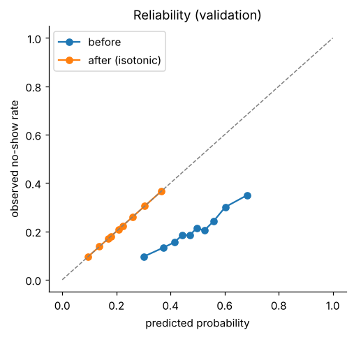
Calibrating on the same data we then plot is optimistic; the honest check comes on the test period below.
Choose the threshold from costs
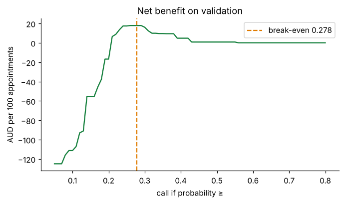
For each possible threshold: how many patients would we call, how many no-shows would we reach, and what is the net benefit per 100 appointments? The break-even threshold from the business case should sit near the top of the curve.
def net_benefit_per_100(y, p, t):
    call = p >= t
    gain = y[call].sum() * CALL_PREVENTS * COST_OF_NO_SHOW - call.sum() * COST_OF_CALL
    return 100 * gain / len(y)


p_val = calibrated.predict_proba(X_val)[:, 1]
yv = y_val.to_numpy()
ts = np.round(np.arange(0.05, 0.81, 0.01), 2)
curve = pd.DataFrame(
    {
        "threshold": ts,
        "call share": [(p_val >= t).mean() for t in ts],
        "no-shows reached": [(p_val[yv == 1] >= t).mean() for t in ts],
        "net benefit per 100": [net_benefit_per_100(yv, p_val, t) for t in ts],
    }
)
fig, ax = plt.subplots(figsize=(7, 3.6))
ax.plot(curve["threshold"], curve["net benefit per 100"], color="#15803D")
ax.axvline(break_even, ls="--", color="#E07B00", label=f"break-even {break_even:.3f}")
ax.set(xlabel="call if probability ≥", ylabel="AUD per 100 appointments", title="Net benefit on validation")
ax.legend()
plt.show()
threshold = break_even
curve.iloc[::5].round(3)
| threshold | call share | no-shows reached | net benefit per 100 | |
|---|---|---|---|---|
| 0 | 0.05 | 0.991 | 0.999 | -124.955 |
| 5 | 0.10 | 0.953 | 0.984 | -111.325 |
| 10 | 0.15 | 0.743 | 0.852 | -55.487 |
| 15 | 0.20 | 0.530 | 0.669 | -16.791 |
| 20 | 0.25 | 0.220 | 0.343 | 17.432 |
| 25 | 0.30 | 0.143 | 0.236 | 16.107 |
| 30 | 0.35 | 0.042 | 0.082 | 9.594 |
| 35 | 0.40 | 0.017 | 0.036 | 4.806 |
| 40 | 0.45 | 0.002 | 0.004 | 0.832 |
| 45 | 0.50 | 0.002 | 0.004 | 0.832 |
| 50 | 0.55 | 0.002 | 0.004 | 0.832 |
| 55 | 0.60 | 0.000 | 0.000 | 0.000 |
| 60 | 0.65 | 0.000 | 0.000 | 0.000 |
| 65 | 0.70 | 0.000 | 0.000 | 0.000 |
| 70 | 0.75 | 0.000 | 0.000 | 0.000 |
| 75 | 0.80 | 0.000 | 0.000 | 0.000 |
Test once
Everything is now fixed: features, model, calibration, threshold. We score the test period a single time and report each metric with a bootstrap 95% confidence interval, plus what the call list would achieve.
X_test, y_test = test[FEATURES], test["no_show"].to_numpy()
p_test = calibrated.predict_proba(X_test)[:, 1]
rng = np.random.default_rng(SEED)
boot = {"ROC-AUC": [], "PR-AUC": []}
for _ in range(1000):
    i = rng.integers(0, len(y_test), len(y_test))
    boot["ROC-AUC"].append(roc_auc_score(y_test[i], p_test[i]))
    boot["PR-AUC"].append(average_precision_score(y_test[i], p_test[i]))
test_scores = scores(y_test, p_test)
report = pd.DataFrame(
    {
        "test": test_scores,
        "95% CI low": {k: np.percentile(v, 2.5) for k, v in boot.items()},
        "95% CI high": {k: np.percentile(v, 97.5) for k, v in boot.items()},
    }
)
report.loc["PR-AUC of baseline", "test"] = y_test.mean()
report.round(4)
| test | 95% CI low | 95% CI high | |
|---|---|---|---|
| ROC-AUC | 0.6181 | 0.6080 | 0.6279 |
| PR-AUC | 0.2941 | 0.2826 | 0.3054 |
| Brier | 0.1604 | NaN | NaN |
| PR-AUC of baseline | 0.2095 | NaN | NaN |
call = p_test >= threshold
summary = pd.Series(
    {
        "share of patients called": call.mean(),
        "share of no-shows reached (recall)": call[y_test == 1].mean(),
        "share of calls that reach a no-show (precision)": y_test[call].mean(),
        "net benefit per 100 appointments, AUD": net_benefit_per_100(y_test, p_test, threshold),
        "net benefit if we call everyone, AUD": net_benefit_per_100(y_test, np.ones_like(p_test), 0.5),
    }
).round(3)
summary
share of patients called                             0.211
share of no-shows reached (recall)                   0.332
share of calls that reach a no-show (precision)      0.329
net benefit per 100 appointments, AUD               19.392
net benefit if we call everyone, AUD              -122.881
dtype: float64
Compare the model with the obvious alternative policy, "call everyone": if that is better, the model is not needed. A positive net benefit that beats calling everyone is the real success measure.
Check fairness
The model must not flag some groups far more often, or miss their no-shows far more, without a good reason. We compare the flag rate and recall of each group with the overall figures and mark any group that differs by more than 25% for review.
rows = []
overall_flag, overall_recall = call.mean(), call[y_test == 1].mean()
for g in ["gender", "age_band", "scholarship"]:
    for value, idx in test.reset_index(drop=True).groupby(g, observed=True).indices.items():
        if len(idx) < 100:
            continue
        yy, ff = y_test[idx], call[idx]
        flag, rec = ff.mean(), ff[yy == 1].mean()
        rows.append(
            {
                "group": g,
                "value": str(value),
                "n": len(idx),
                "no-show rate": yy.mean(),
                "flag rate": flag,
                "recall": rec,
                "review": not (0.8 <= flag / overall_flag <= 1.25 and 0.8 <= rec / overall_recall <= 1.25),
            }
        )
fairness = pd.DataFrame(rows)
fairness.round(3)
| group | value | n | no-show rate | flag rate | recall | review | |
|---|---|---|---|---|---|---|---|
| 0 | gender | F | 12448 | 0.211 | 0.215 | 0.335 | False |
| 1 | gender | M | 6668 | 0.207 | 0.205 | 0.326 | False |
| 2 | age_band | 0-12 | 2426 | 0.254 | 0.443 | 0.585 | True |
| 3 | age_band | 13-17 | 1853 | 0.262 | 0.341 | 0.458 | True |
| 4 | age_band | 18-34 | 6052 | 0.227 | 0.258 | 0.376 | False |
| 5 | age_band | 35-49 | 3812 | 0.190 | 0.141 | 0.217 | True |
| 6 | age_band | 50-64 | 2363 | 0.182 | 0.070 | 0.118 | True |
| 7 | age_band | 65+ | 2610 | 0.145 | 0.027 | 0.058 | True |
| 8 | scholarship | 0 | 17212 | 0.204 | 0.189 | 0.302 | False |
| 9 | scholarship | 1 | 1904 | 0.258 | 0.417 | 0.545 | True |
Groups marked for review need a human decision, not an automatic fix: a group with a genuinely higher no-show rate will be flagged more often. What matters is that the extra calls help (a reminder is not a penalty) and that the model is never used to deny care.
Explain the model
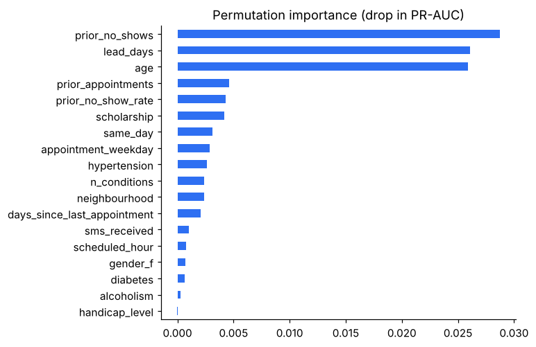
Permutation importance (on validation, not test): how much PR-AUC drops when a feature is shuffled. Partial dependence: how the average prediction changes with one feature.
from sklearn.inspection import PartialDependenceDisplay, permutation_importance

sample = val.sample(5000, random_state=SEED)
imp = permutation_importance(
    calibrated,
    sample[FEATURES],
    sample["no_show"],
    scoring="average_precision",
    n_repeats=5,
    random_state=SEED,
    n_jobs=-1,
)
importance = pd.Series(imp.importances_mean, index=FEATURES).sort_values()
fig, ax = plt.subplots(figsize=(6, 5))
importance.plot.barh(ax=ax, color="#2E6FF2")
ax.set(title="Permutation importance (drop in PR-AUC)", xlabel="")
plt.show()
fig, axes = plt.subplots(1, 3, figsize=(12, 3.4))
PartialDependenceDisplay.from_estimator(
    calibrated,
    sample[FEATURES].astype({c: "float64" for c in NUMERIC}),
    ["lead_days", "age", "prior_no_show_rate"],
    ax=axes,
    grid_resolution=30,
)
fig.tight_layout()
plt.show()
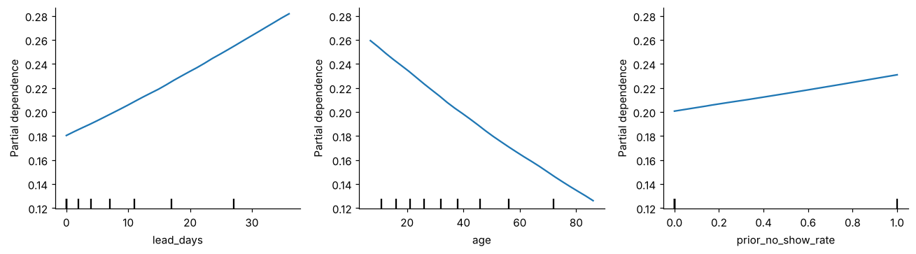
Check the story against common sense: risk should rise with lead time and with past no-shows. A surprising top feature is often a sign of leakage, so this step doubles as a final leak check.
Save the model
Save the model with everything needed to use it correctly: the threshold, the feature list and versions.
import joblib
import sklearn

bundle = {
    "model": calibrated,
    "threshold": float(threshold),
    "features": FEATURES,
    "model_name": best_name,
    "sklearn": sklearn.__version__,
    "validation_start": str(validation_start.date()),
    "test_start": str(test_start.date()),
}
Path("models").mkdir(exist_ok=True)
joblib.dump(bundle, "models/noshow_model.joblib")
print("saved models/noshow_model.joblib")
saved models/noshow_model.joblib
From notebook to production
This notebook is the project: it is where the answer was found. If the clinic wants the call list every day,
a notebook is not enough: it has to run unattended, be tested on every change, and answer requests from the booking
system. So the next step is to move this notebook's code, unchanged, into a Python package with tests, an API and
monitoring. The reference repository for this project (p01-noshow.zip) shows the result:
| notebook section | moves to | tested by |
|---|---|---|
| Check data quality | src/noshow/data/schema.py |
tests/test_data.py |
| Clean the data | src/noshow/data/clean.py |
tests/test_data.py |
| Split by time | src/noshow/features/split.py |
tests/test_features.py |
| Engineer features | src/noshow/features/build.py |
tests/test_features.py (including leakage) |
| Models | src/noshow/models/pipelines.py, train.py |
tests/test_model_and_api.py |
| Test, fairness, explain | src/noshow/evaluation/report.py → MODEL_CARD.md |
tests/test_metrics.py |
| Use the model | src/noshow/serving/app.py (API), Dockerfile |
tests/test_model_and_api.py |
Moving code must not change results. When this notebook sits inside that repository, the next cell proves it: the package's cleaning and features give the same table, and its model with our tuned settings gives the same predictions. On its own (for example in Colab), the cell simply skips.
try:
    from noshow.data.clean import clean as pkg_clean
    from noshow.features.build import FEATURES as PKG_FEATURES
    from noshow.features.build import build_features as pkg_build_features
    from noshow.models.pipelines import build as pkg_build
except ImportError:
    print("the production package is not installed here, so the comparison is skipped")
else:
    pkg_clean_df, _ = pkg_clean(raw, max_age=115)
    pd.testing.assert_frame_equal(pkg_clean_df, clean)
    pd.testing.assert_frame_equal(
        pkg_build_features(pkg_clean_df).reset_index(drop=True), feats.reset_index(drop=True)
    )
    assert PKG_FEATURES == FEATURES
    name = {"logistic": "logistic", "gradient boosting": "hist_gradient_boosting"}[best_name]
    best_params = {"logistic": search_lr, "gradient boosting": search_hgb}[best_name].best_params_
    pkg_model = pkg_build(name, SEED).set_params(**best_params).fit(X_train, y_train)
    np.testing.assert_allclose(pkg_model.predict_proba(X_val)[:, 1], best.predict_proba(X_val)[:, 1])
    print("notebook and production package agree: same clean data, same features, same predictions")
notebook and production package agree: same clean data, same features, same predictions
In the repository, the whole pipeline then runs from a terminal:
make all      # validate -> prepare -> eda -> train -> evaluate, writes reports/MODEL_CARD.md
make test     # 42 tests
make serve    # the prediction API on http://127.0.0.1:8000
What you built
- A problem framed by its decision and costs, with a threshold set before modelling.
- Clean, validated data, split by time, with history features that cannot leak the future.
- A baseline, two tuned models, calibration, one honest test with confidence intervals.
- A fairness check, explanations and a saved model, and proof that the production code matches the notebook.
Try next: add the number of days until the appointment's weekday holiday; change the costs and watch the threshold move; compare isotonic with sigmoid calibration.
Run the whole pipeline with one command
In the package, each notebook section became a command, so anyone can rebuild the model from raw data in one go and get the same
result: make all runs validate, prepare, EDA, train and evaluate, and writes reports/MODEL_CARD.md. Settings live in
configs/config.yaml instead of notebook variables.
Makefile54 lines
# One command per pipeline step. Run `make help` to list them.
PY ?= python
CONFIG ?= configs/config.yaml

.PHONY: help install data synthetic validate prepare eda train evaluate report serve test lint typecheck check all clean docker

help:          ## List the available commands
	@grep -E '^[a-z-]+:.*## ' Makefile | sed 's/:.*## /\t/'

install:       ## Install pinned dependencies and the package in editable mode
	$(PY) -m pip install -r requirements-dev.txt && $(PY) -m pip install -e . --no-deps && pre-commit install

data:          ## Download the real dataset from Kaggle (needs a Kaggle API token)
	$(PY) -m noshow.cli download --config $(CONFIG)

synthetic:     ## Create a full-size synthetic dataset with the same schema (no account needed)
	$(PY) scripts/make_synthetic.py --rows 110527 --out data/raw/noshowappointments-kagglev2-may-2016.csv

validate:      ## Check the raw data against the schema
	$(PY) -m noshow.cli validate --config $(CONFIG)

prepare:       ## Clean the data and build point-in-time features
	$(PY) -m noshow.cli prepare --config $(CONFIG)

eda:           ## Write the exploratory data analysis report and figures
	$(PY) -m noshow.cli eda --config $(CONFIG)

train:         ## Tune and train the candidate models, select the best, calibrate it
	$(PY) -m noshow.cli train --config $(CONFIG)

evaluate:      ## Final test-set evaluation, fairness, explanations and model card
	$(PY) -m noshow.cli evaluate --config $(CONFIG)

all: validate prepare eda train evaluate   ## Run the whole pipeline

serve:         ## Run the prediction API locally
	$(PY) -m flask --app noshow.serving.app run --debug --port 8000

test:          ## Run the test suite
	$(PY) -m pytest

lint:          ## Lint and check formatting
	ruff check . && ruff format --check .

typecheck:     ## Static type checks
	mypy

check: lint typecheck test   ## Everything CI runs

docker:        ## Build the serving image
	docker build -t noshow-api .

clean:         ## Remove generated data, models and reports
	rm -rf data/interim/* data/processed/* models/* reports/* runs/*
configs/config.yaml50 lines
# All settings for the no-show project. Change values here, never in code.
project:
  name: noshow
  seed: 42

paths:
  raw_csv: data/raw/noshowappointments-kagglev2-may-2016.csv
  interim: data/interim/appointments_clean.parquet
  features: data/processed/features.parquet
  model_dir: models
  reports: reports
  runs: runs

data:
  kaggle_dataset: joniarroba/noshowappointments
  expected_rows_min: 100000        # the real file has 110,527 rows; fail loudly if far off
  max_age: 115                     # ages above this are treated as data-entry errors

split:
  # Time-based: train on the earliest appointments, validate and test on later ones,
  # exactly as the model would be used (trained on the past, scoring the future).
  validation_fraction: 0.15
  test_fraction: 0.15
  cv_folds: 5                      # GroupKFold by patient inside the training period

features:
  history_min_days_gap: 1          # only appointments that finished at least 1 day before scheduling count as history
  neighbourhood_min_frequency: 50  # rarer neighbourhoods are grouped as "other" in the linear model

training:
  primary_metric: average_precision   # PR-AUC: the positive class (no-show) is the minority
  tuning_iterations: 20
  candidate_models: [dummy, logistic, hist_gradient_boosting]

decision:
  # Assumptions to agree with the clinic before deployment (see docs/problem_framing.md).
  cost_of_call: 5.0                # staff time for one reminder call, AUD
  cost_of_no_show: 60.0            # value of a wasted appointment slot, AUD
  call_prevents_no_show_rate: 0.30 # share of would-be no-shows that a call turns into attendance
  max_calls_per_day: null          # optional capacity limit

evaluation:
  bootstrap_samples: 1000
  calibration_bins: 10
  fairness_groups: [gender, age_band, scholarship]
  fairness_max_ratio: 1.25         # flag a group whose recall or flag rate differs by more than 25% from the overall

monitoring:
  psi_warn: 0.10
  psi_alert: 0.25
Test what the notebook showed
The checks you did by eye in the notebook become 42 automated tests that run on every change: cleaning rules, the leakage check, time periods that never overlap, folds that never share patients, model behaviour (more past no-shows never lowers risk), training-serving parity and the API contract.
tests/test_features.py: the leakage check as a test12 lines
def test_history_uses_only_outcomes_known_at_booking() -> None:
    h = history_features(_toy(), min_days_gap=1)
    # Booking made on 3 May: only the 1 May appointment had happened. The 5 May outcome is in the
    # future at booking time and must NOT be counted (that would be leakage).
    assert h.loc[2, "prior_appointments"] == 1
    assert h.loc[2, "prior_no_shows"] == 1
    assert h.loc[2, "prior_no_show_rate"] == 1.0
    assert h.loc[2, "days_since_last_appointment"] == 2
    # First appointments have no history
    assert h.loc[0, "prior_appointments"] == 0 and np.isnan(h.loc[0, "prior_no_show_rate"])
    # Patients never share history
assert h.loc[3, "prior_appointments"] == 0Serve predictions with an API
The clinic's booking system asks for predictions over HTTP. The Flask app loads the saved model once, validates every request, and returns each probability with the decision (call or not), the threshold and the model version. Logs never contain personal data.
src/noshow/serving/schemas.py: the request contract32 lines
class Appointment(BaseModel):
    """One upcoming appointment, plus the patient's history from the clinic database."""

    model_config = ConfigDict(extra="forbid")

    appointment_id: int = Field(gt=0)
    scheduled_at: datetime = Field(description="When the booking was made")
    appointment_date: date
    age: int = Field(ge=0, le=115)
    gender: Literal["F", "M"]
    neighbourhood: str = Field(min_length=1, max_length=100)
    scholarship: bool = False
    hypertension: bool = False
    diabetes: bool = False
    alcoholism: bool = False
    handicap_level: int = Field(default=0, ge=0, le=4)
    sms_received: bool = False
    prior_appointments: int = Field(
        default=0, ge=0, description="Earlier appointments with a recorded outcome"
    )
    prior_no_shows: int = Field(default=0, ge=0)
    days_since_last_appointment: int | None = Field(default=None, ge=0)

    @model_validator(mode="after")
    def _consistent(self) -> Appointment:
        if self.appointment_date < self.scheduled_at.date():
            raise ValueError("appointment_date is before the booking date")
        if self.prior_no_shows > self.prior_appointments:
            raise ValueError("prior_no_shows cannot exceed prior_appointments")
        if (self.prior_appointments == 0) != (self.days_since_last_appointment is None):
            raise ValueError("days_since_last_appointment must be given exactly when prior_appointments > 0")
return selfsrc/noshow/serving/app.py79 lines
def create_app(model_path: str | Path | None = None) -> Flask:
    """Application factory: loads the model bundle once at start-up."""
    app = Flask(__name__)
    app.config["MAX_CONTENT_LENGTH"] = MAX_BODY_BYTES
    path = Path(model_path or os.environ.get("MODEL_PATH", "models/model.joblib"))
    bundle: dict[str, Any] = joblib.load(path)
    model, threshold, version = bundle["model"], float(bundle["threshold"]), str(bundle["version"])
    logging.basicConfig(level=logging.INFO, format="%(asctime)s %(levelname)s %(name)s: %(message)s")
    log.info("loaded model %s from %s", version, path)

    @app.before_request
    def _start() -> None:
        g.t0, g.request_id = time.perf_counter(), request.headers.get("X-Request-ID", uuid.uuid4().hex[:12])

    @app.after_request
    def _finish(resp: Response) -> Response:
        resp.headers["X-Request-ID"] = g.request_id
        resp.headers["X-Model-Version"] = version
        log.info(
            "request_id=%s %s %s status=%s ms=%.1f",
            g.request_id,
            request.method,
            request.path,
            resp.status_code,
            (time.perf_counter() - g.t0) * 1000,
        )
        return resp

    @app.get("/health")
    def health() -> Response:
        return jsonify(status="ok", model_version=version)

    @app.post("/v1/predict")
    def predict() -> tuple[Response, int]:
        body = request.get_json(silent=True)
        if body is None:
            return jsonify(
                error="invalid_json", message="send a JSON body with Content-Type: application/json"
            ), 400
        try:
            req = PredictRequest.model_validate(body)
        except ValidationError as e:
            problems = [
                {"field": ".".join(map(str, err["loc"])), "message": err["msg"]} for err in e.errors()
            ]
            return jsonify(error="invalid_request", problems=problems), 422
        probs = model.predict_proba(to_features(req))[:, 1]
        resp = PredictResponse(
            model_version=version,
            threshold=threshold,
            predictions=[
                Prediction(
                    appointment_id=a.appointment_id,
                    no_show_probability=round(float(p), 4),
                    recommend_call=bool(p >= threshold),
                )
                for a, p in zip(req.appointments, probs, strict=True)
            ],
        )
        # Log only ids, scores and the version: no personal data in logs.
        log.info(
            "request_id=%s scored=%d flagged=%d", g.request_id, len(probs), int((probs >= threshold).sum())
        )
        return jsonify(resp.model_dump()), 200

    @app.errorhandler(404)
    def not_found(_: Exception) -> tuple[Response, int]:
        return jsonify(error="not_found", message="see /health and /v1/predict"), 404

    @app.errorhandler(413)
    def too_large(_: Exception) -> tuple[Response, int]:
        return jsonify(error="payload_too_large", message=f"limit is {MAX_BODY_BYTES} bytes"), 413

    @app.errorhandler(500)
    def server_error(_: Exception) -> tuple[Response, int]:
        log.exception("request_id=%s failed", getattr(g, "request_id", "?"))
        return jsonify(error="internal_error", message="the error has been logged"), 500

return appDocker and continuous integration
The Docker image holds only the API and the model and runs as a non-root user. On every push, CI runs lint, strict type checks, all tests and the whole pipeline on synthetic data; a red build blocks merging.
Dockerfile28 lines
# Serving image: only the API and the trained model, nothing else.
FROM python:3.12-slim

ENV PYTHONDONTWRITEBYTECODE=1 \
    PYTHONUNBUFFERED=1 \
    PIP_NO_CACHE_DIR=1

WORKDIR /app

COPY requirements.txt .
RUN pip install -r requirements.txt gunicorn==23.0.0

COPY pyproject.toml README.md ./
COPY src ./src
RUN pip install --no-deps .

# The trained, calibrated model bundle produced by `make train` (copied in at build time).
COPY models/model.joblib /app/models/model.joblib
COPY configs ./configs

RUN useradd --create-home --uid 10001 appuser
USER appuser

ENV MODEL_PATH=/app/models/model.joblib \
    PORT=8000
EXPOSE 8000
HEALTHCHECK --interval=30s --timeout=3s CMD python -c "import urllib.request,os; urllib.request.urlopen(f'http://127.0.0.1:{os.environ[\"PORT\"]}/health')"
CMD gunicorn --workers 2 --bind 0.0.0.0:$PORT --access-logfile - "noshow.serving.app:create_app()"
.github/workflows/ci.yml28 lines
name: ci
on:
  push:
  pull_request:

jobs:
  check:
    runs-on: ubuntu-latest
    steps:
      - uses: actions/checkout@v4
      - uses: actions/setup-python@v5
        with:
          python-version: "3.12"
          cache: pip
      - name: Install
        run: |
          python -m pip install -r requirements-dev.txt
          python -m pip install -e . --no-deps
      - name: Lint
        run: ruff check . && ruff format --check .
      - name: Type check
        run: mypy
      - name: Tests (synthetic data, no Kaggle account needed)
        run: python -m pytest --cov=noshow --cov-report=term-missing
      - name: Pipeline smoke run on synthetic data
        run: |
          python scripts/make_synthetic.py --rows 20000 --out data/raw/noshowappointments-kagglev2-may-2016.csv
          make all CONFIG=configs/ci.yaml
Monitor and retrain
After launch, watch input drift (Population Stability Index per feature against the training data), the share of patients flagged, and real
performance once outcomes arrive. python -m noshow.cli monitor exits with code 2 on an alert so a scheduled job fails loudly.
docs/monitoring.md: retraining policy6 lines
## Retraining policy
1. **Trigger:** scheduled every 3 months, or earlier when a monitoring alert is confirmed by real outcomes.
2. **Data:** all appointments up to the cut-off, with the newest period held out as the test set.
3. **Same gates as the first release:** tests pass, beats the baseline, calibration checked, fairness review signed.
4. **Shadow first:** the candidate scores live traffic for one week without affecting calls; compare with the live model.
5. **Release:** switch `MODEL_PATH`; keep the previous bundle. **Rollback** = point `MODEL_PATH` back and restart.Present it in your portfolio
- Link the notebook first: it tells the story. Then the model card and the repository.
- Show the net-benefit chart: it turns a model score into money.
- In interviews, talk about the leakage you prevented, why the threshold comes from costs, and what the fairness table showed.